Substitution of variables

In mathematics, substitution of variables (also called variable substitution or coordinate transformation) refers to the substitution of certain variables with other variables. Though the study of how variable substitutions affect a certain problem can be interesting in itself, they are often used when solving mathematical or physical problems, as the correct substitution may greatly simplify a problem which is hard to solve in the original variables. Under certain conditions the solution to the original problem can be recovered by back-substitution (inverting the substitution).

1 Formal introduction
2 Common examples
3 Lagrangian mechanics
4 See also

Formal introduction

Let $A$ , $B$ be smooth manifolds and let $\Phi: A \rightarrow B$ be a $C^r$ -diffeomorphism between them, that is: $\Phi$ is a $r$ times continuously differentiable, bijective map from $A$ to $B$ with $r$ times continuously differentiable inverse from $B$ to $A$ . Here $r$ may be any natural number (or zero), $\infty$ (smooth) or $\omega$ (analytic).

The map $\Phi$ is called a regular coordinate transformation or regular variable substitution, where $regular$ refers to the $C^r$ -ness of $\Phi$ . Usually one will write $x = \Phi(y)$ to indicate the replacement of the variable $x$ by the variable $y$ by substituting the value of $\Phi$ in $y$ for every occurrence of $x$ .

Common examples

Cylindrical coordinates

Some systems can be more easily solved when switching to cylindrical coordinates. Consider for example the equation

$U(x, y, z)�:= (x^2 %2B y^2) \sqrt{ 1 - \frac{x^2}{x^2 %2B y^2} } = 0.$

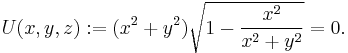
This may be a potential energy function for some physical problem. If one does not immediately see a solution, one might try the substitution

$\displaystyle (x, y, z) = \Phi(r, \theta, z)$ given by $\displaystyle \Phi(r, \theta, z) = (r \cos(\theta), r \sin(\theta), z)$ .

Note that if $\theta$ runs outside a $2\pi$ -length interval, for example, $[0, 2\pi]$ , the map $\Phi$ is no longer bijective. Therefore $\Phi$ should be limited to, for example $(0, \infty] \times [0, 2\pi) \times [-\infty, \infty]$ . Notice how $r = 0$ is excluded, for $\Phi$ is not bijective in the origin ( $\theta$ can take any value, the point will be mapped to (0, 0, z)). Then, replacing all occurrences of the original variables by the new expressions prescribed by $\Phi$ and using the identity $\sin^2 x %2B \cos^2 x = 1$ , we get

$V(r, \theta, z) = r^2 \sqrt{ 1 - \frac{r^2 \cos^2 \theta}{r^2} } = r^2 \sqrt{1 - \cos^2 \theta} = r^2 \sin\theta$ .

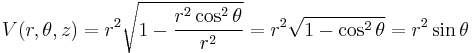Now the solutions can be readily found: $\sin(\theta) = 0$ , so $\theta = 0$ or $\theta = \pi$ . Applying the inverse of $\Phi$ shows that this is equivalent to $y = 0$ while $x \not= 0$ . Indeed we see that for $y = 0$ the function vanishes, except for the origin.

Note that, had we allowed $r = 0$ , the origin would also have been a solution, though it is not a solution to the original problem. Here the bijectivity of $\Phi$ is crucial.

Integration

Main article: Integration by substitution

Under the proper variable substitution, calculating an integral may become considerably easier. Consult the main article for an example.

Momentum vs. velocity

Consider a system of equations

$m \dot v = - \frac{ \partial H }{ \partial x }$

$m \dot x = \frac{ \partial H }{ \partial v }$

for a given function $H(x, v)$ . The mass can be eliminated by the (trivial) substitution $\Phi(p) = 1/m \cdot v$ . Clearly this is a bijective map from $\mathbb{R}$ to $\mathbb{R}$ . Under the substitution $v = \Phi(p)$ the system becomes

$\dot p = - \frac{ \partial H }{ \partial x }$

$\dot x = \frac{ \partial H }{ \partial p }$

Lagrangian mechanics

Main article: Lagrangian mechanics

Given a force field $\phi(t, x, v)$ , Newton's equations of motion are

$m \ddot x = \phi(t, x, v)$ .

Lagrange examined how these equations of motion change under an arbitrary substitution of variables $x = \Psi(t, y)$ , $v = \frac{\partial \Psi(t, y)}{\partial t} %2B \frac{\partial\Psi(t, y)}{\partial y} \cdot w$ .

He found that the equations

$\frac{ \partial{L} }{ \partial y} = \frac{\mathrm{d}}{\mathrm{d}t} \frac{\partial{L}}{\partial{w}}$

are equivalent to Newton's equations for the function $L = T - V$ , where T is the kinetic, and V the potential energy.

In fact, when the substitution is chosen well (exploiting for example symmetries and constraints of the system) these equations are much easier to solve than Newton's equations in Cartesian coordinates.